Image sizes in an R markdown Document

At Jumping Rivers we recently moved our website from WordPress to Hugo. The main reason for the move was that since the team are all very comfortable with Git, continuous integration and continuous development using a static web-site generator made more sense than WordPress. Additional benefits are decreasing the page loading time speed and general site security - WordPress sites are notorious for getting hacked if not kept up to date.

While thinking about WordPress brings a host of painful memories, one of the benefits was it does (sort of) hide the pain of optimising images for web-pages. There are numerous WordPress plugins that manipulate, cache and optimise the delivery of your graphics. Of course, this is also a potential security problem, but that’s another story. When we ported over our pages, we noticed that the graphics on blog posts and course descriptions were all slightly different. The images had different resolutions, file formats and dimensions. While they all looked OK, they certainly weren’t standardised or optimised!

In this series of posts we’ll consider the (simple?) task of generating and including figures for the web using R & {knitr}. Originally this was going to be a single post, but as the length increase, we’ve decided to separate it into a separate articles. The four posts we intend to cover are

• setting the image size (this post)
• selecting the image type, PNG vs JPEG vs SVG
• including non-generated files in a document
• setting global {knitr} options.

Before we go further, these series of articles are all aimed at web documents. How we handle PDFs is slightly different and will be covered at a different time. Also, I’m trying optimise images for the web, but at the same time, I’m not going to chase down every last byte to shave off a milli-second on page-speeds.

It’s also worth reading our previous post on generating consistent graphs in R across different operating systems.

Do you use RStudio Pro? If so, checkout out our managed RStudio services

What Makes Figures Special

There’s lots of information on the web on how to optimise images for websites. Figures like line graphs, scatter plots and histograms, have to be handled a little differently than pictures. Graphs have a few distinctive characteristics.

As they usually contain text, this means we have to pay specific attention to image quality. Also, while we can resize a photograph easily, resizing a graph with text may make the axis unreadable. Furthermore, images contain thin lines and perhaps use opacity within the plot.

The core problem we are trying to solve is when we create a web page (a HTML file), the page gives a containing box with a certain width and height. We want to create a figure that matches these dimensions.

If the figure we create is too large for the box, the browser (or some clever server-side plugin) will resize your image. This has two downsides

• if the client downloads the image, this will increase your page loading speed
• if the figure contains text, then the text will become smaller

If the figure is smaller than the box, then your figure will look pixelated and the text may become unreadable.

The DPI issue

If you’ve ever Googled web-graphics before, you will have come across DPI or dots per inch. The typical recommendation for web-graphics is 72dpi. However, this is completely the wrong way of thinking about it. When you put a graphic/image on a website, you have a set number of pixels. This is the unit of measurement you need to consider when generating a graphic. If you are generating a graph for a PDF, then DPI is important as you can cram more points in a space. However, on a monitor you have pixels.

If your web-designer tells you to provide a 600px by 600px image - that’s what they need. DPI doesn’t actually come into this calculation!

The one caveat to the above (as we’ll see) is that dpi alters the text size when creating R images.

Setting image dimensions

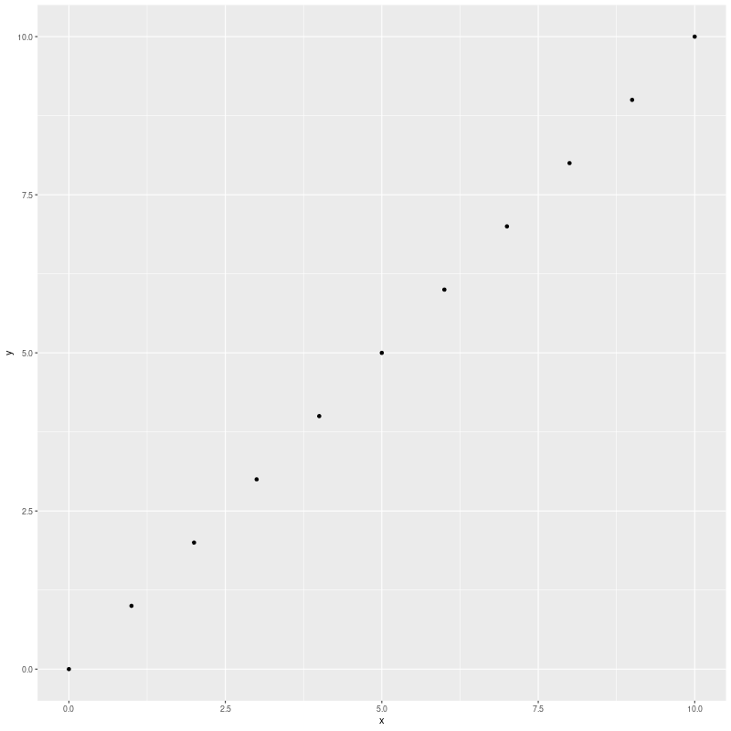
If you are creating graphics using the png() function (or a similar graphics device), then you simply need to specify the dimensions using the width and height arguments. As an example, let’s create a simple {ggplot2} scatter plot

library("ggplot2")
dd = data.frame(x = 0:10, y = 0:10)
g = ggplot(dd, aes(x, y)) + 
  geom_point()

which we then save with dimensions of 400px by 400px:

png("figure1-400.png", width = 400, height = 400, type = "cairo-png")
g
dev.off()

This creates a perfectly sized 400px by 400px image

# As we'll see below, we may have to double this resolution
# for retina displays
dim(png::readPNG("figure1-400.png", TRUE))
#> [1] 400 400

When we include the scatter plot

knitr::include_graphics("figure1-400.png")

it comes out at the perfect size and resolution.

The graphics Goldilocks principle

Suppose we create images that aren’t the correct size for the HTML container. Is it really that bad? If we create an image double the size, 800px by 800px,

png("figure1-800.png", width = 800, height = 800, type = "cairo-png")
g
dev.off()

and try and squeeze it into a 400px box. The font size becomes tiny. The “quality” of the figure is fine, it’s just unreadable.

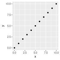
If we create an image that is only 200px, and then expanded it to fit the 400px container box, the text becomes too large and the graph is fuzzy.

png("figure1-200.png", width = 200, height = 200, type = "cairo-png")
g
dev.off()

Instead, we need something not too big, not too small. But something that just fits.

Setting sizes in {knitr}

At Jumping Rivers, most of the time we create graphs for HTML pages it’s performed within an R markdown document via {knitr}. Above, we created images by specifying the exact number of pixels. However in {knitr} you can’t specify the number of pixels when creating the image, instead you set the figure dimensions and also the output dimensions. The image units are hard-coded as inches within {knitr}.

The dimensions of the image are calculated via fig.height * dpi and fig.width * dpi. The fig.retina argument also comes into play, but we’ll set fig.retina = 1, which will match above, then come back to this idea at the end.

If we want to create an image with dimensions d1 and d2, then we set the {knitr} chunks to

• fig.width = d1 / 72,
• fig.width = d2 / 72
• dpi = 72 - the default
• fig.retina = 1
• dev.args = list(type = "cairo-png") - not actually needed, but you should set it!

In theory, you should be able to set dpi to anything and get the same image, but the dpi value is passed to the res argument in png(), and that controls the text scaling. So changing dpi means your text changes. In practice, leave dpi at the default value. If you want to change the your text size, then change them in your plot.

But what about out.width and out.height?

The {knitr} arguments out.width and out.height don’t change the dimensions of the png created. Instead, they control the size of the HTML container on the web-page. As we seen above, we want the container size to match the image size. By default this should happen, but you can specify the sizes explicitly out.width = "400px".

But what about fig.retina?

When fig.retina is set to 2, the dpi is doubled, but the display sized is halved. The practical result of this is:

• file sizes increase, so page loading also increases
• anyone with a retina display will see a crisper graph
• if someone zooms into the plot on the browser, the graph should still look nice even at 200% magnification.

The defaults for fig.retina differ between {rmarkdown} and {knitr}. So rather than trying to figure it out, set it explicitly at the top of the document via

## Or 1 if you want
knitr::opts_chunk$set(fig.retina = 2)

Whether you set it to 1 or 2 doesn’t affect the values you set for dpi and fig. What it does affect is the size of the generated image. If you don’t believe me, create two images and examine the dimensions with the png::readPNG() function.

But what about fig.asp?

The chunk argument fig.asp controls the aspect ratio of the plot. For example, setting fig.width = fig.height would give an aspect ratio of 1. Consequently, you would only ever define two of fig.width, fig.height and fig.asp.

Typically I set fig.asp = 0.7 in the {knitr} header, ignore fig.height and specify the fig.width in each chunk as needed.

Is that all?

Unfortunately not. The following three graphics have all been using exactly the same {knitr} chunk options

• fig.width = 400/72 and fig.height = 400/72

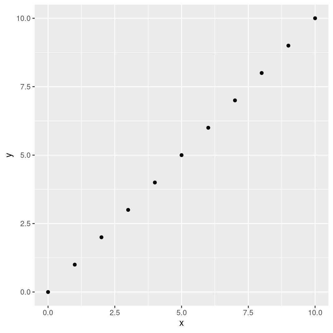
This has been our running {ggplot2} example

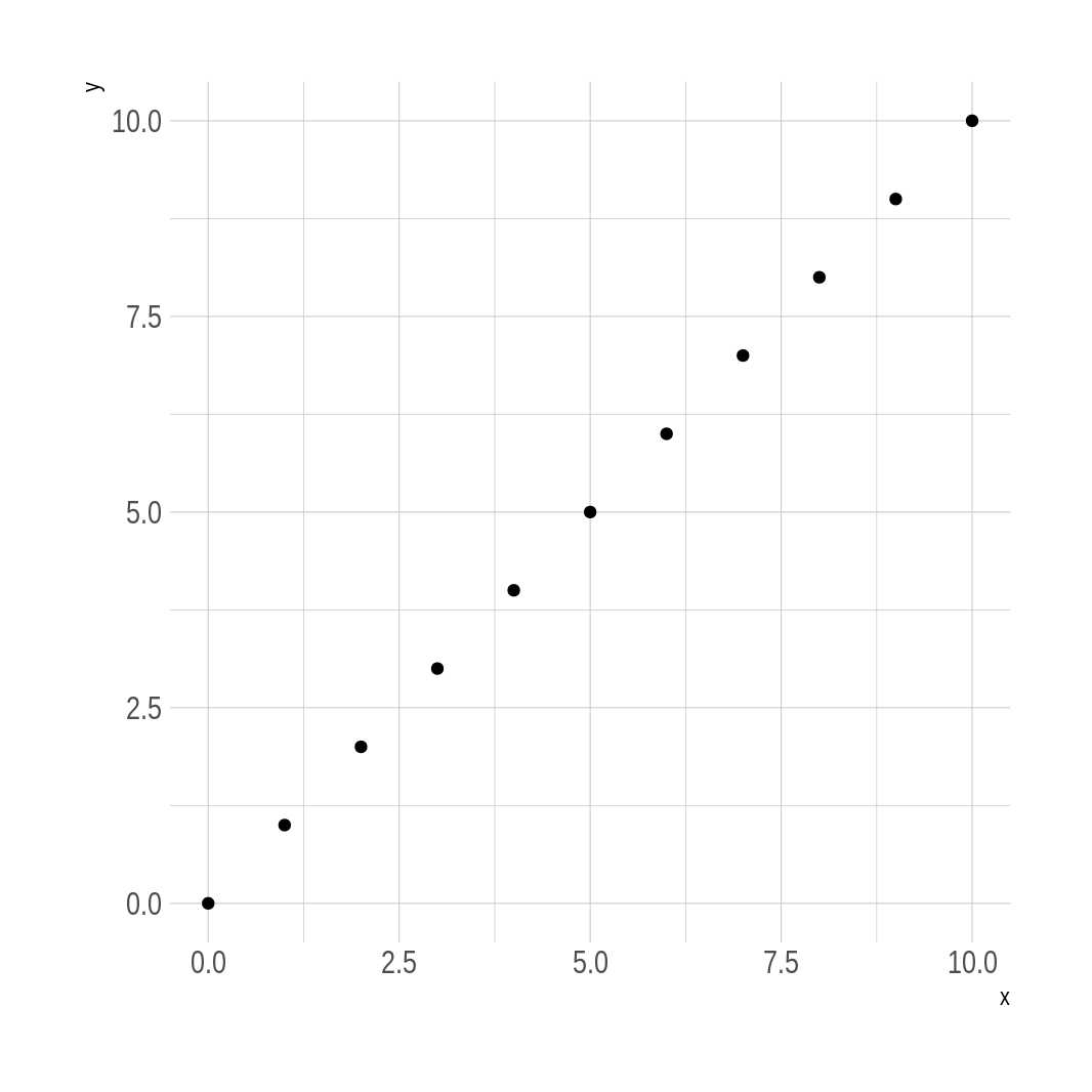
This is changing the theme via hrbrthemes::theme_ipsum()

g + hrbrthemes::theme_ipsum()

and this is standard base graphics

plot(dd$x, dd$y)

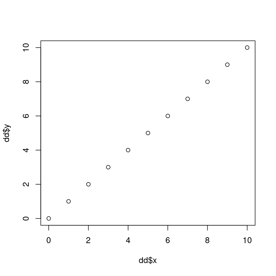
Notice that the latter two plots have a larger white space border around them. You could use a tool to automatically crop the white space, but that changes the dimensions of the image. Instead, you should use some R code to remove the surrounding white space.