Comparing plotly & ggplotly plot generation times

The {plotly} package. A godsend for interactive documents, dashboard and presentations. For such documents, there is no doubt that anyone would prefer a plot created in {plotly} rather than {ggplot2}. Why? Using {plotly} gives you neat and crucially interactive options at the top, whereas {ggplot2} objects are static. In an app we have been developing here at Jumping Rivers, we found ourselves asking the question would it be quicker to use plot_ly() or wrapping a {ggplot2} object in ggplotly()? I found the results staggering.

Prerequisites

Throughout we will be using the packages: {dplyr}, {tidyr}, {ggplot2}, {plotly} and {microbenchmark}. The data in use is the birthdays dataset in the {mosaicData} package. This data sets contains the daily birth count in each state of the USA from 1969 - 1988. The packages can be installed in the usual way (remember you can install packages in parallel)

install.packages(c("mosaicData", "dplyr", "tidyr",
                  "ggplot2", "plotly", "microbenchmark"))
library("mosaicData")
library("dplyr")
library("tidyr")
library("ggplot2")
library("plotly")
library("microbenchmark")

Analysis

Let’s load and take a look at the data.

data("Birthdays", package = "mosaicData")
head(Birthdays)
##   state year month day       date wday births
## 1    AK 1969     1   1 1969-01-01  Wed     14
## 2    AL 1969     1   1 1969-01-01  Wed    174
## 3    AR 1969     1   1 1969-01-01  Wed     78
## 4    AZ 1969     1   1 1969-01-01  Wed     84
## 5    CA 1969     1   1 1969-01-01  Wed    824
## 6    CO 1969     1   1 1969-01-01  Wed    100

First, we’ll create a very simple scatter graph of the mean births in every year.

meanb = Birthdays %>%
    group_by(year) %>%
    summarise(mean = mean(births))

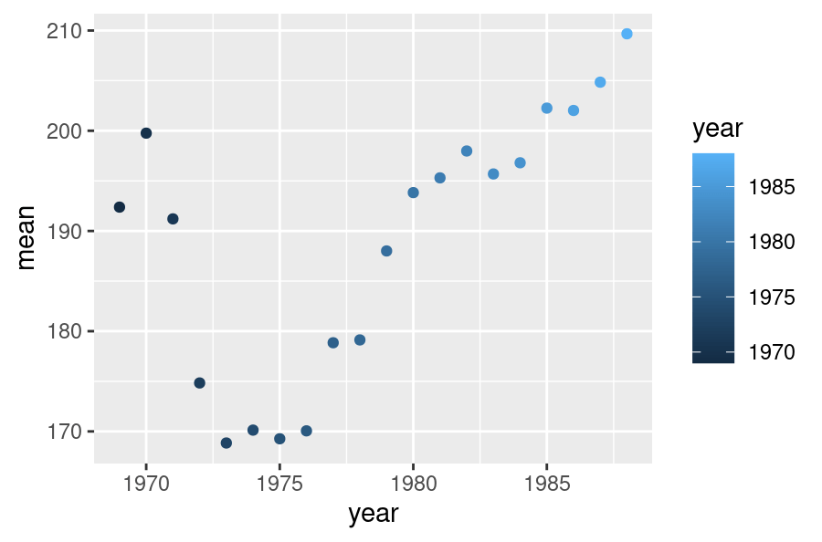
Wrapping this as a {ggplot2} object inside ggplotly() we obtain this…

ggplotly(ggplot(meanb) +
  geom_point(aes(y = mean, x = year, colour = year)))

Whilst using plot_ly() give us this…

plot_ly(data = meanb,
        y = ~mean, x = ~year, color = ~year,
        type = "scatter")

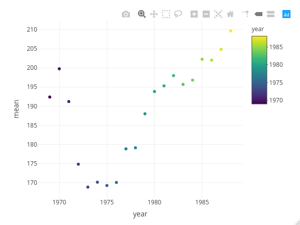
Both graphs are, identical, bar styling, yes? Now let’s use {microbenchmark} to see how their timings compare (for an overview of timing R functions, see our previous blog post).

time = microbenchmark::microbenchmark(
        ggplotly = ggplotly(ggplot(meanb) +
                            geom_point(aes(y = mean, x = year, colour = year))),
        plotly = plot_ly(data = meanb,
                         y = ~mean, x = ~year,
                         color = ~year, type = "scatter"),
        times = 100, unit = "s")
time
## Unit: seconds
##      expr      min       lq     mean   median       uq     max neval cld
##  ggplotly 0.050139 0.052229 0.070750 0.054760 0.056785 1.56652   100   b
##    plotly 0.002475 0.002527 0.003017 0.002571 0.002674 0.03061   100  a
autoplot(time)

Now I thought nesting a {ggplot} object within ggplotly() would be slower than using plot_ly(), but I didn’t think it would be this slow. On average ggplotly() is approximately 23 times slower than plot_ly(). 23!

Let’s take it up a notch. There we were plotting only 20 points, what about if we plot over 20,000? Here we will plot the min, mean and max births on each day.

date = Birthdays %>%
  group_by(date) %>%
  summarise(mean = mean(births), min = min(births), max = max(births)) %>%
  gather(birth_stat, value, -date)

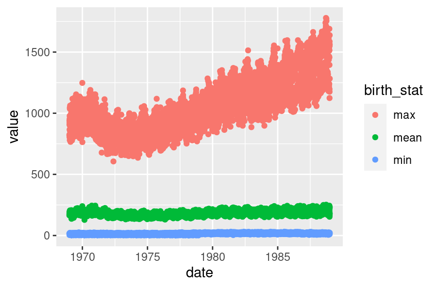
Wrapping this a {ggplot2} object inside ggplotly() we obtain this graph…

ggplotly(ggplot(date) +
    geom_point(aes(y = value, x = date, colour = birth_stat)))

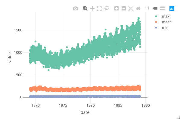
Whilst using plot_ly() we obtain…

plot_ly(date,
        x = ~date, y = ~value, color = ~birth_stat,
        type = "scatter")

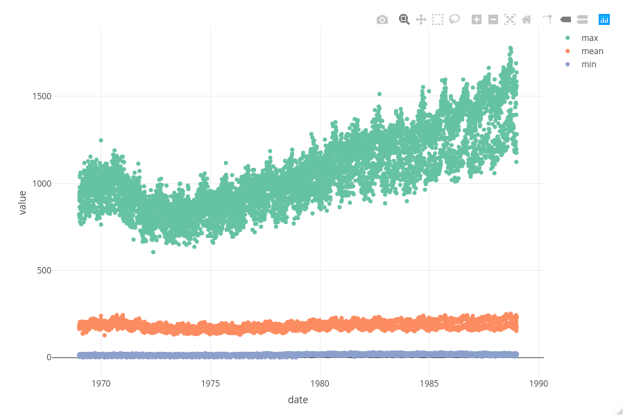
Again, both plots are identical, bar styling.

time2 = microbenchmark(
  ggplotly = ggplotly(
    ggplot(date) +
      geom_point(aes(y = value, x = date, colour = birth_stat))
    ),
    plotly = plot_ly(date, x = ~date, y = ~value,
                      color = ~birth_stat,
                      type = "scatter"),
  times = 100, unit = "s")
time2
## Unit: seconds
##      expr      min       lq     mean   median       uq     max neval cld
##  ggplotly 0.335823 0.355301 0.389759 0.365353 0.378502 0.54746   100   b
##    plotly 0.002472 0.002534 0.002719 0.002585 0.002675 0.01179   100  a
autoplot(time2)

On average ggplotly() is 143 times slower than plot_ly(), with the max run time being 0.547 seconds!

Summary

I’m going to level with you. Using ggplotly() in interactive mode isn’t a problem. Well, it’s not a problem until your shiny dashboard or your markdown document has to generate a few plots at the same time. With only one plot, you’ll probably go with the method that gives you your style in the easiest way possible and you’ll do this with no repercussions. However, let’s say you’re making a shiny dashboard and it now has over 5 interactive graphs within it. Suddenly, if you’re using ggplotly(), the lag we noticed in the analysis above starts to build up unnecessarily. That’s why I’d use plot_ly().

Thanks for chatting!

R.version.string
## [1] "R version 3.4.2 (2017-09-28)"
packageVersion("ggplot2")
## [1] '2.2.1'
packageVersion("plotly")
## [1] '4.7.1'