
Timing hash functions with the bench package
Published: May 21, 2019

This blog post has two goals
- Investigate the {bench} package for timing R functions
- Consequently explore the different algorithms in the {digest} package using {bench}
What is {digest}?
The {digest} package provides a hash function to summarise R objects. Standard hashes are available, such as md5, crc32, sha-1, and sha-256.
The key function in the package is digest() that applies a cryptographical hash function to arbitrary R objects. By default, the objects are internally serialized using md5. For example,
library("digest")
digest(1234)
## [1] "37c3db57937cc950b924e1dccb76f051"
digest(1234, algo = "sha256")
## [1] "01b3680722a3f3a3094c9845956b6b8eba07f0b938e6a0238ed62b8b4065b538"
The {digest} package is fairly popular and has a large number of reverse dependencies
length(tools::package_dependencies("digest", reverse = TRUE)$digest)
## [1] 186
The number of available hashing algorithms has grown over the years, and as a little side project, we decided to test the speed of the various algorithms. To be clear, I’m not considering any security aspects or the potential of hash clashes, just pure speed.
Timing in R
There are numerous ways of timing R functions. A recent addition to this list is the {bench} package. The main function bench::mark() has a number of useful features over other timing functions.
To time and compare two functions, we load the relevant packages
library("bench")
library("digest")
library("tidyverse")
then we call the mark() function and compare the md5 with the sha1 hash
value = 1234
mark(check = FALSE,
     md5 = digest(value, algo = "md5"),
     sha1 = digest(value, algo = "sha256")) %>%
  select(expression,  median)
## # A tibble: 2 x 2
##   expression   median
##   <bch:expr> <bch:tm>
## 1 md5          50.2µs
## 2 sha1         50.9µs
The resulting tibble object, contains all the timing information. For simplicity, we’ve just selected the expression and median time.
More advanced {bench}
Of course, it’s more likely that you’ll want to compare more than two things. You can compare as many function calls as you want with mark(), as we’ll demonstrate in the following example. It’s probably more likely that you’ll want to compare these function calls against more than one value. For example, in the {digest} package there are eight different algorithms. Ranging from the standard md5 to the newer xxhash64 methods. To compare times, we’ll generate n = 20 random character strings of length N = 10,000. This can all be wrapped up in the single function press() function call from the {bench} package:
N = 1e4
results = suppressMessages(
  bench::press(
    value = replicate(n = 20, paste0(sample(LETTERS, N, replace = TRUE), collapse = "")),
    {
      bench::mark(
        iterations = 1, check = FALSE,
        md5      = digest(value, algo = "md5"),
        sha1     = digest(value, algo = "sha1"),
        crc32    = digest(value, algo = "crc32"),
        sha256   = digest(value, algo = "sha256"),
        sha512   = digest(value, algo = "sha512"),
        xxhash32 = digest(value, algo = "xxhash32"),
        xxhash64 = digest(value, algo = "xxhash64"),
        murmur32 = digest(value, algo = "murmur32")
      )
    }
  )
)
The tibble results contain timing results. But it’s easier to work with relative timings. So we’ll rescale
rel_timings = results %>%
  unnest() %>%
  select(expression, median) %>%
  mutate(expression = names(expression)) %>%
  distinct() %>%
  mutate(median_rel = unclass(median/min(median)))
Then plot the results, ordered by slowed to largest
ggplot(rel_timings) +
  geom_boxplot(aes(x = fct_reorder(expression, median_rel), y = median_rel)) +
  theme_minimal() +
  ylab("Relative timings") + xlab(NULL) +
  ggtitle("N = 10,000") + coord_flip()
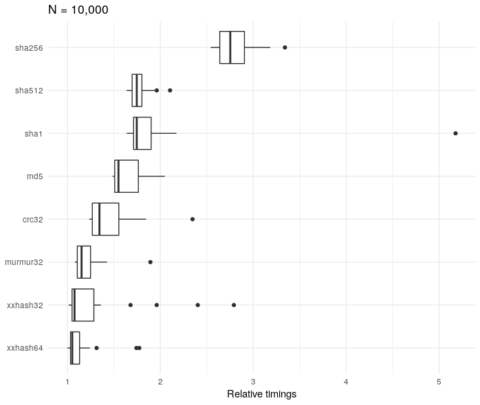
The sha256 algorithm is about three times slower than the xxhash32 method. However, it’s worth bearing in mind that although it’s relatively slower, the absolute times are very small
rel_timings %>%
  group_by(expression) %>%
  summarise(median = median(median)) %>%
  arrange(desc(median))
## # A tibble: 8 x 2
##   expression   median
##   <chr>      <bch:tm>
## 1 sha256      171.2µs
## 2 sha1        112.6µs
## 3 md5         109.5µs
## 4 sha512      108.4µs
## 5 crc32          91µs
## 6 xxhash64     85.1µs
## 7 murmur32     82.1µs
## 8 xxhash32     77.6µs
It’s also worth seeing how the results vary according to the size of the character string N.
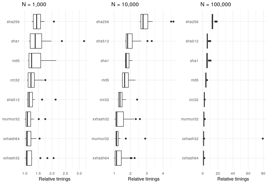
Regardless of the value of N, the sha256 algorithm is consistently in the slowest.
Conclusion
R is going the way of “tidy” data. Though it wasn’t the focus of this blog post, I think that the {bench} package is as good as other timing packages out there. Not only that, but it fits in with the whole “tidy” data thing. Two birds, one stone.